
This article first appeared in Data Science Briefings, the DataMiningApps newsletter. Subscribe now for free if you want to be the first to receive our feature articles, or follow us @DataMiningApps. Do you also wish to contribute to Data Science Briefings? Shoot us an e-mail over at briefings@dataminingapps.com and let’s get in touch!
Structurally Advancing the Strategic Impact of Credit Risk Management Through The “Optimal Credit Portfolio Curve”
Contributed by Joris Peeters, Chief Data Scientist & Strategic Consultant at Altares
Introduction
For individual companies as well as on a macroeconomic level, granting credit is a critical factor for success, growth and driving business forward. Doing so, however, also entails a degree of risk as the borrower or beneficiary of the credit line may not be able to repay at the end of the term, causing a financial loss for the creditor. Through the setting of credit limits, companies can control how much risk they are willing to take on a given customer or counterparty. However, due to their risk limiting effect, credit limits also limit sales and revenue. Furthermore, the inherent slowness of the classical credit limit decisioning process often impacts the overall customer experience and may even render a digital strategy, futile. Therefore, “the credit limit” is a natural source of debate and conflict between C-level executives, sales teams and credit/finance teams.
Over the past decades, we have supported quite some companies in automating their B2B credit limit decision process. Hereby, next to credit scores and ratings, we introduced the use of specific ML models to calculate an appropriate credit limit, to drive the RPA and make the process inherently ‘intelligent’ [1]. Combined with electronic data flows, these models helped to make their credit limit setting process far more efficient and productive. This in turn opened the possibility to drive digital strategies, create unique customer experiences and even revamp entire back-office structures. In short, it pushed their business on another level.
As we progressed through this RPA journey, we found ourselves confronted with the quest for what the “optimal credit limits” would be, and achieve this with the ML models. To this end, we developed a theoretical Risk-Reward based framework, allowing a practical determination of the most optimal credit limits through the Optimal Credit Portfolio Curve.
This article describes the Optimal Credit Portfolio Curve theory, reflecting R&D work we did on credit limits. Part I details the derivation of the Optimal Credit Portfolio Curve on a portfolio of credit limits. Part II provides an overview of additional control metrics, designed to overcome overexposure and to add human control. Part III describes the strategic implications of using the Optimal Portfolio Curve. The last part concludes the article [2].
Part I – The efficient credit portfolio curve
Fundamental to the Optimal Portfolio Curve theory, is the trade-off between Risk (financial losses from non-payment on a business transaction) and Reward (profit made from a successful business transaction). Surely, credit limit decisions are bound to be different given the unique product market combination at any given company, but additionally we experienced first-hand how the risk appetite of a company strongly influences the credit limit outcome. Typically, we can see three broad classifications of companies on risk appetite: (1) risk averse, (2) neutral, and (3) risk taking.
As an illustration, consider the example in Figure 1 below, showing the evolution of a credit limit setting for the three above-mentioned risk appetite categories. The horizontal axis is Time. The Y-axis is the amount of credit limit granted to a particular buyer, in Euros. The financial performance of the buyer is expressed by the credit rating, which in this example deteriorates over time, with the business ultimately going into a default.
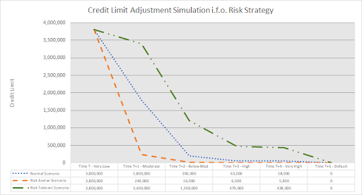
Fig. 1 Risk Appetite and Credit Limit Setting
On Time T, the 3 risk appetite profiles each have a credit limit of 3.8 million Euro, given an assessment that the risk of default is very low. However, as the credit rating drops over time, all three risk profiles lower their credit limit, but at a very different pace. The Risk Neutral and Risk Averse profiles converge to a very low limit, already well before the default of the buyer. The Risk Tolerant profile in contract maintains a higher credit limit for an extended period and may eventually suffer a higher credit loss.
We rely on machine learning and mathematical models to generate credit limits for individual buyers. However, to integrate the risk appetite parameters into these models, and to help a company set appropriate risk appetite parameters, we leveraged insights from the portfolio management theories in the capital markets. Particularly the concepts of the Capital Assets Pricing Model and the Efficient Portfolio Curve from Markowitz [3].
Similar to the modern portfolio management concepts, we started to view the buyers of a company as a group of investment assets. Other than in the capital markets, where the evolution of the stock market indices and the price of individual stocks are key buildings blocks, our model focusses on how changes in the risk appetite parameters generate revenue and profit, versus potential credit losses or a total credit cost.
Linking this back to Fig. 1 above, this shows just three possible outcomes of the credit limit formula. However, by changing the risk appetite parameters in our ML credit limit model, a wide variety of credit limits can be generated. As each credit limit translates into sales, it also generates profit. This is the Reward side of the equation. The potential losses represent the Risk side of the equation. This could be expressed as an Expected Loss type of calculation, or as a total cost of credit, depending on the underlying calculation.
By calculating a credit limit and expected loss for each counterparty in a portfolio, an aggregated view can be generated on (1) how much credit is granted, and therefore how much sales and profit can be realized, and (2) what the total cost of credit or the total expected losses would be. This allows to run a Monte Carlo type analysis, whereby – albeit between a set of boundaries – the computer iteratively selects a different set of risk appetite parameters, each resulting in an alternative aggregated portfolio outcome of Risk and Reward.
Figure 2 below depicts the result of such a Monte Carlo simulation, for 20.000 iterations, ran on a portfolio of credit limits. The X-axis represents the total credit limit volume (‘Reward’). The Y-axis shows the total expected loss (‘Risk’). Each blue dot represents the aggregated outcome of the Reward, and the corresponding Risk. The orange dot represents the current Risk-Reward situation.

Fig. 2 Simulation Results of Total Credit Limit Volume vs Expected Loss
Interestingly, the resulting outcome demonstrates that for each given ‘Reward’ total (i.e. the X-axis in Fig. 2), there exists a range of possible outcomes for the Risk (in this case expressed as the Expected Loss). The reason for this is due to the way the risk parameters interact with the underlying ML models, resulting in a different spreading of the credit limits across the buyer portfolio [4], and as such resulting in different loss levels.
From this analysis, the optimal, or efficient portfolio curve can be easily extracted: this curve is the collection of risk appetite parameters which for a given total aggregated credit volume, give the lowest level of credit losses. Fig. 3 below shows the Optimal or Efficient Portfolio Curve, for a range of 10.000 simulations ran across the same buyer portfolio used for Fig. 2 above.
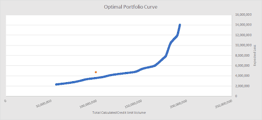
Fig. 3 Optimal or Efficient Portfolio Curve
Once the framework has been established, additional dimensions can be added to the simulations. Consider for example the addition of a forward-looking component on the Credit Rating or Credit Score Model. In order to simulate the impact of a change in PD level on the Optimal Portfolio Curve, we leveraged the insights gained from a PD level Beta assessment which we ran on a time series of the PD levels per the D&B Rating Risk Indicator, against the GDP evolution in the Netherlands.
When applying these Beta factors to the Risk model underpinning the credit limit system and choosing a macro-economic outlook, a new forward-looking adjusted optimal portfolio curve is generated. Figure 4 below depicts the outcome of the simulation, for a scenario with a less favorable macro-economic outlook. The blue dots are from the original simulation. The grey dots provide the post-stressed combinations of Risk-Reward and essentially provide a new optimal portfolio curve.
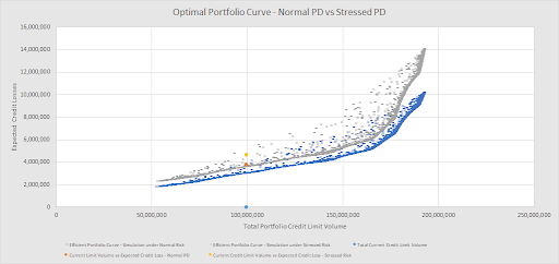
Fig. 4 Optimal Portfolio Curve with ‘stressed’ PD values
Part II – Additional Control Metrics
When developing the ML based credit limit systems, the underlying credit limits as (historically) set by the credit team are used as [one of] the dependent variables(s). As these limits were often influenced by business and strategic considerations, the model(s) outcome(s) may also reflect these latter, and cause what we refer to as ‘localized overexposure’.
Additionally, whilst the goal of the portfolio curve is to determine the most optimal credit limits, few are willing to adopt the ML-derived outcomes without first gaining a clear understanding of how these calculated limits align or deviate from the existing credit limits. These latter serve as a benchmark or comparison basis, on which the performance or the ML models will always be judged.
Lastly, as indicated above, the total credit limit volume is represented by the ‘Reward’, whilst the ‘Risk’ is represented by the expected loss. If a profit level per customer is available – which is not always easy to obtain – , then this enables the possibility of off-setting total limit volume against profit levels.
For the first two points above, we expanded the ML/AI models and the Optimal Portfolio Curve to include two additional control components:
- A maximum exposure ML model, which controls credit worthiness as well as the size of the business. Again, parametrizable so as take risk appetite into consideration.
- A distribution index metric which provides a summary of the degree by which the credit limit distribution generated by a set of Risk-Reward parameters, is dis-/similar from the original credit limit distribution.
On the third point, we ran a simulation based on assumed profitability levels. Figure 7 provides an indication of the relationship between the distribution index and the assumed profit margin. It shows clearly that a lower distribution index correlates with a higher overall profit margin [5]. This does, however, not automatically translate into a higher overall Euro profit number, as most of these less creditworthy customers are also typically smaller companies in nature. The total credit limit volume and total profit would therefore be reduced for these scenarios, making them probably less preferable for senior management.
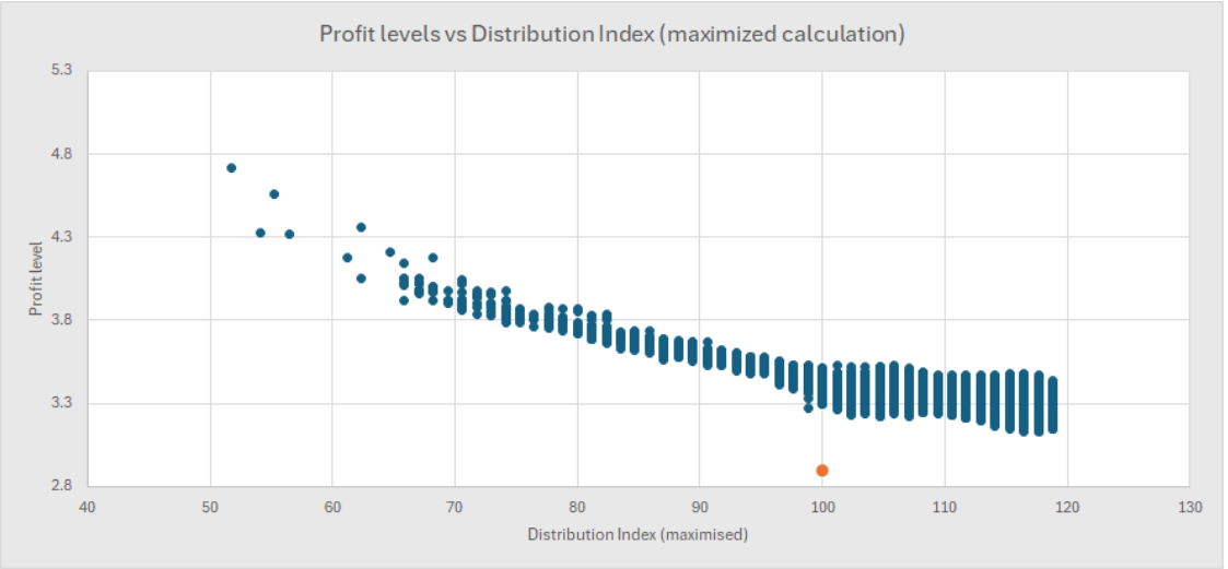
Fig. 5 Profit margin level versus Distribution Index (maximized)
Part III – Strategic implications
Companies leveraging ML and/or AI models to automate a large part of their credit decisioning process, ultimately possess a powerful tool to increase the effectiveness, efficiency and productivity of their internal processes, enhance the customer experience, and structurally drive top-line and bottom-line results. We have seen it. We have experienced it.
Over and above these benefits, the Optimal Credit Portfolio theory presented above, provides a highly practical framework allowing companies to choose the optimal balance between Risk and Reward, in line with the company’s strategic turnover and profit goal, and with the risk appetite of the executive C-level and – ultimately – the shareholders.
The total ML system allows sales and finance/credit teams to jointly prepare which scenarios provide credit limits that would support the revenue growth opportunities identified by the sales team. If this happens, credit limits become effectively Risk Adjusted Customer Lifetime Value assessments.
One word of caution however is at its place here: operationally, successfully deploying such systems for the long run requires a fundamental change in both the thought- and the operational processes in the organization. Only those companies who embrace this fundamental shift will enjoy the full, long-lasting benefit.
Conclusion
Based upon the development of effective and efficient ML systems to drive automation in credit risk management, our work around the quest for the most optimal credit limits resulted in a solid framework, enabling strategic Risk-Reward choices.
Leveraging, but also adjusting to our needs and objectives, the insights from the capital markets, notably the Markowitz optimal portfolio theory and the CAPM models, our approach resulted in the Optimal or Efficient Portfolio Curve. This curve represents the combinations of Risk and Reward, where for each Reward, the Risk is minimized. Or, alternatively, for a given Risk, the most optimal Reward can be chosen.
Used well, the framework provides credit/finance and sales teams with a solid basis for intense cooperation, proactively combining future sales opportunities with proactive credit limit setting, aligned with the risk appetite, strategic goals, and objectives of the company.
Ultimately, our goal was to create a solid theoretical framework for strategic credit limit setting, combining Risk and Reward. With our Optimal Credit Portfolio Curve, we feel we have structurally advanced towards that objective. Much remains to be researched and optimized, for sure. But for now, we can effectively support companies by turning traditionally reactive credit limits into strategic, pro-active Risk Adjusted Customer Credit Lifetime Value assessments.
Notes
[1] A typical sought-after balance was/is to achieve 80% of credit requests to be processed automatically, and 20% to be assessed manually.
[2] The article does not provide an overview or description of the underlying credit score or credit limit ML or AI models, nor for the Risk-Reward formula. Of course, the more optimal these models are, the more insightful the output of the Optimal Portfolio Curve will be.
[3] For example, on https://quantpedia.com/markowitz-model/
[4] The underlying ML models follow a solid subject matter and mathematical logic. The risk appetite parameters interact with these models, but as follows from Fig 1, a more risk tolerant attitude results in higher credit limits awarded. As such, the underlying structure and logic of how credit limits are assigned does not alter when changing the risk appetite parameters, but the overall limit size per buyer may increase (risk tolerant) or decrease (risk averse) in function of the risk appetite parameters chosen.
[5] One of the assumptions made for this analysis, was the typical inverted relationship between profit margins and creditworthiness, partially explaining the output of this analysis.