Contributed by: Bart Baesens
This article first appeared in Data Science Briefings, the DataMiningApps newsletter. Subscribe now for free if you want to be the first to receive our feature articles, or follow us @DataMiningApps. Do you also wish to contribute to Data Science Briefings? Shoot us an e-mail over at briefings@dataminingapps.com and let’s get in touch!
Introduction
In recent decades, the use of social media websites in everybody’s daily life is booming. People can continue their conversations on social networking sites like Facebook, Twitter, LinkedIn, Google+, Instagram, etc., and share their experiences with their acquaintances, friends, family, etc. It takes only one click to update your whereabouts to the rest of the world. There are plenty of options to broadcast your current activities: by a picture, video, geo-location, links, or just plain text.
Users of online social networking sites explicitly reveal their relationships with other people. Consequently, social networking sites are a nearly perfect mapping of the relationships that exist in the real world. They know who you are, what your hobbies and interests are, to whom you are married, how many children you have, your buddies with whom you run every week, your friends of the wine club, etc. This massively interconnected network of people knowing each other in some way is an extremely interesting source of information and knowledge. Marketing managers no longer need to guess who might influence whom to create the appropriate campaign. It is all there….which is the problem. Social networking sites acknowledge the richness of the data sources they have and are not willing to share them free of cost. Those data are often privatized and regulated, and well-hidden from commercial use. On the other hand, social networking sites offer many built-in facilities to managers and other interested parties to launch and manage their marketing campaigns by exploiting the social network, without publishing the exact network representation.
However, companies often forget that they can reconstruct a portion of the social network using in-house data. Telecommunication providers, for example, have a massive transactional database where they record call behavior of their customers. Under the assumption that good friends call each other more often, we can recreate the network and indicate the tie strength between people based on the frequency and/or duration of calls. Internet infrastructure providers might map the relationships between people using their customers’ IP-addresses. IP-addresses that frequently communicate are represented by a stronger relationship. In the end, the IP-network will envisage the relational structure between people from another point of view, but to a certain extent, as observed in reality. Many more examples can be found in the banking, retail and online gaming industries. In this article, we discuss how social networks can be leveraged for analytics.
Social Network Definitions
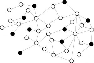
A social network consists of both nodes (vertices) and edges. Both must be clearly defined at the outset of the analysis. A node (vertex) could be defined as a customer (private/professional), household/family, patient, doctor, paper, author, terrorist, webpage, … An edge can be defined as a friend’s relationship, a call, transmission of a disease, a ‘follows’ relationship, a reference, etc. Note that the edges can also be weighted based upon interaction frequency, the importance of information exchange, intimacy, emotional intensity, and so on. For example: in a churn prediction setting, the edge can be weighted according to the (total) time two customers called each other during a specific period. Social networks can be represented as a sociogram. This is illustrated in the below figure whereby the color of the nodes corresponds to a specific status (e.g., churner or non-churner).
 Example sociogram.
Sociograms are useful for representing small-scale networks. For large-scale networks, the network is typically represented as a matrix (see below). These matrices will be symmetrical [1] and typically very sparse (with lots of zeros). The matrix can also contain the weights if weighted connections occur.
| C1 | C2 | C3 | C4 | |
| C1 | – | 1 | 1 | 0 |
| C2 | 1 | – | 0 | 1 |
| C3 | 1 | 0 | – | 0 |
| C4 | 0 | 1 | 0 | – |
Matrix representation of a social network.
In what follows, we discuss how social networks can be leveraged for both descriptive and predictive analytics.
Descriptive Analytics: Social Network Metrics and Community Mining
Remember, the aim of descriptive analytics is to describe a data set using a set of key statistics or metrics. A social network can be characterized by various centrality metrics. The most important centrality measures are depicted in the below table.
| Geodesic | Shortest path between two nodes in the network. |
| Degree | Number of connections of a node (in- versus out-degree if the connections are directed). |
| Closeness | The average distance of a node to all other nodes in the network (reciprocal of farness). |
| Betweenness | Counts the number of times a node or edge lies on the shortest path between any two nodes in the network. |
| Graph theoretic center | The node with the smallest maximum distance to all other nodes in the network. |
Common network centrality measures.
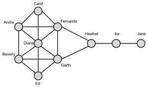
These metrics can now be illustrated with the Kite network toy example depicted in the below figure [2]:

The Kite network.
| Degree | Closeness | Betweenness | |||
| 6 | Diane | 0.64 | Fernando | 14 | Heather |
| 5 | Fernando | 0.64 | Garth | 8.33 | Fernando |
| 5 | Garth | 0.6 | Diane | 8.33 | Garth |
| 4 | Andre | 0.6 | Heather | 8 | Ike |
| 4 | Beverly | 0.53 | Andre | 3.67 | Diane |
| 3 | Carol | 0.53 | Beverly | 0.83 | Andre |
| 3 | Ed | 0.5 | Carol | 0.83 | Beverly |
| 3 | Heather | 0.5 | Ed | 0 | Carol |
| 2 | Ike | 0.43 | Ike | 0 | Ed |
| 1 | Jane | 0.31 | Jane | 0 | Jane |
Centrality measures for the Kite network.
The above table reports the centrality measures for the Kite network. Based on degree, Diane is most central since she has the most connections. She works as a connector, or hub. Note, however, that she only connects those already connected to each other. Fernando and Garth are the closest to all others. They are the best positioned to communicate messages that must flow quickly through to all other nodes in the network. Heather has the highest betweenness. She sits between two important communities (Ike and Jane versus the rest). She plays a broker role between both communities, but is also a single point of failure. Note that the betweenness measure is often used for community mining. A popular technique here is the Girvan-Newman algorithm which works as follows [3]:
- The betweenness of all existing edges in the network is calculated first.
- The edge with the highest betweenness is removed.
- The betweenness of all edges affected by the removal is recalculated.
- Steps 2 and 3 are repeated until no edges remain.
The result is essentially a dendrogram (similar to e.g. hierarchical clustering), which can then be used to decide upon the optimal number of communities. Community mining serves various purposes. It allows understanding the behavior of homogeneous subsets in your network which can be especially relevant in marketing analytics (e.g. for targeted recommendations) or fraud detection (to detect e.g. fraud rings). Furthermore, community information can also be leveraged for predictive analytics, by using e.g. featurization procedures as we discuss below.
Predictive Analytics: Social Network Learning
In predictive analytics, the aim is to measure a target variable of interest. Examples could be churn, fraud, default, or customer lifetime value (CLV). In social network learning, the goal is to compute the class membership probability (e.g., churn probability) of a specific node, given the status of the other nodes in the network. Various important challenges arise when learning in social networks. A key challenge is that the data are not independent and identically distributed (IID), an assumption often made in classical statistical models (e.g., linear and logistic regression). The correlational behavior between nodes implies that the class membership of one node might influence the class membership of a related node. Next, it is not easy to come up with a split into a training set for model development and a test set for model validation, since the whole network is interconnected and cannot just be cut into two parts. Moreover, many networks are huge in scale (e.g., a call graph from a telecom provider), and efficient computational procedures need to be developed to do the learning. Finally, one should not forget the traditional way of doing analytics using only node-specific information (i.e., without the network aspects) since this can still be very valuable information for prediction as well.
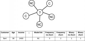
A straightforward way to leverage social networks for predictive analytics is by summarizing the network in a set of features which can then be combined with non-network (i.e., local) characteristics for predictive modeling. A popular example of this is relational logistic regression as introduced by Lu and Getoor (2003) [4]. This approach basically starts off from a data set with local node-specific characteristics and adds network features to it as follows:
- Most frequently occurring class of neighbor (mode-link);
- Frequency of the classes of the neighbors (frequency-link);
- Binary indicators indicating class presence (binary-link).
This is illustrated in the below figure for customer Bart.
Relational logistic regression.
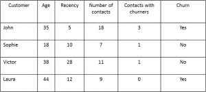
A logistic regression model or decision tree can then be estimated using the data set with both local and network characteristics. Note there is some correlation between the network characteristics added, which should be filtered out during an input selection procedure. Creating network features is also called featurization, since the network characteristics are basically added as special features to the data set. These features can measure the behavior of the neighbors in terms of the target variable (e.g., churn or not) or in terms of the local node-specific characteristics (e.g., age, promotions, etc.). The below figure provides an example in which a feature is added describing the number of contacts with churners. The final column labelled ‘Churn’ is the target variable.
Example of featurization with features describing target behavior of neighbors.
The below figure provides an example where features are added describing the local node behavior of the neighbors.
Example of featurization with features describing local node behavior of neighbors.
Privacy
Obviously, the use of social network data for analytical purposes also requires a thorough reflection on privacy. Customers are often times unaware of their data traces both on-line and off-line and how they can be analyzed. Hence, especially under the current GDPR regulation, it is of key importance that firms always properly disclose what data they gather and how they use it. When doing so, they should not only focus on potential privacy treats but also on customer benefits such that customers can make a well-informed decision about if, when and how their data can be used.
Conclusion
In this article, we zoomed in on social network analytics. We started off by providing key social network definitions. We then illustrated how social networks can be leveraged for descriptive analytics by summarizing them by means of social network metrics such as closeness, betweenness, etc. Next, we elaborated on using social networks for predictive analytics using various featurization procedures. It is important to note that although social networks represent a new type of information, one should definitely not overestimate their power. More specifically, one should not abandon traditional, non-network data for doing analytics. Throughout our research, we found that the best analytical models for e.g. churn prediction are fraud detection are typically built using a combination of both network and non-network data. Finally, it is important to note that whenever analyzing social network data, privacy should always be respected!
References and notes
- [1] Note that this is only the case for undirected networks. For directed networks, representing e.g. a ‘follows’ relationship that is not necessarily reciprocal, the matrix will not be symmetrical.
- [2] Krackhardt, D, Assessing the Political Landscape: Structure, Cognition, and Power in Organizations, Administrative Science Quarterly, 35, pp. 342-369, 1990.
- [3] Girvan M., Newman M. E. J., Community structure in social and biological networks, Proceedings of the National Academy of Sciences, USA 99, pp. 7821–7826, 2002.
- [4] Lu Q., Getoor L., Link-based Classification, Proceeding of the Twentieth Conference on Machine Learning (ICML-2003), Washington DC, 2003.


