Contributed by: Michael Reusens, Wilfried Lemahieu, Bart Baesens
This article first appeared in Data Science Briefings, the DataMiningApps newsletter. Subscribe now for free if you want to be the first to receive our feature articles, or follow us @DataMiningApps. Do you also wish to contribute to Data Science Briefings? Shoot us an e-mail over at briefings@dataminingapps.com and let’s get in touch!
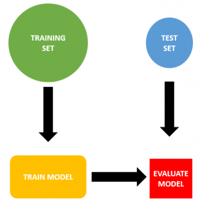
Typically, when training a predictive model, the data is split in a training and a test set. The model is trained by optimizing a performance metric (accuracy, AUROC, …) on the training set. Once a model is trained on the training set, it is evaluated on the test set. Training the model on one set and evaluating it on another makes sure that the model generalizes to unseen data, and does not only work well for the training set.
 |
Intuitively it makes sense that a model is only valuable when it performs better than random guessing. Let’s take a look at the small example below:
 |
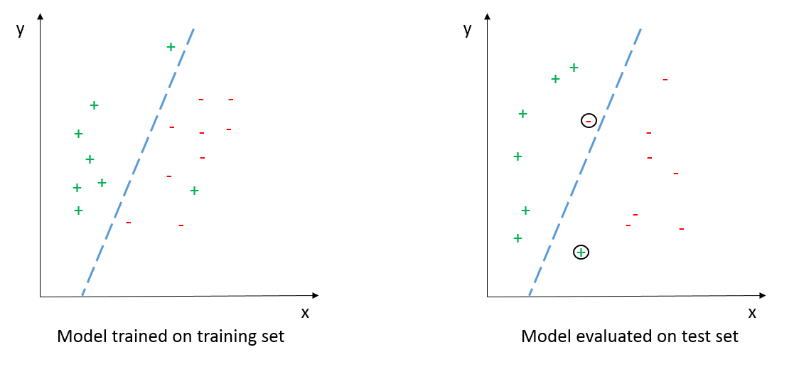
A simple linear classifier is trained on the training set, maximizing the training set accuracy to 94% (left side: 16/17 examples are correctly classified). The model is then evaluated on the test set, resulting in an accuracy of 88% (right side: 14/16). This is a simple example of how training a model on a training set, and using it to predict the labels of unseen examples works quite well. The predictions made on the unseen examples are clearly better than random guessing, which would result in a 50% accuracy on average (AUC = 0.5).
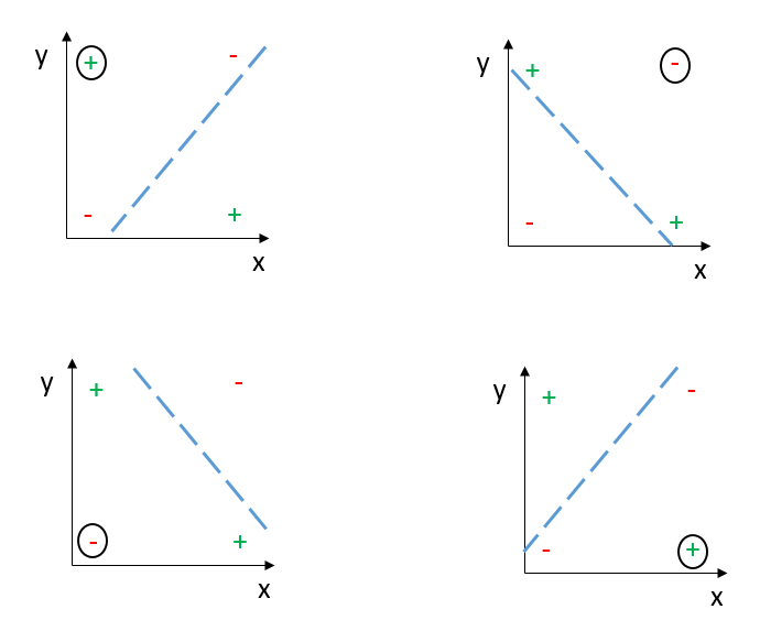
However, in some cases, it is possible that the model accuracy on the test set is consistently worse than random guessing (AUC < 0.5). The most basic example of this is trying to make a linear classifier for XOR data, as shown below. Training a linear model (the dashed blue line) on 3 out of the 4 data points will always result in the misclassification of the test set (the circled observations). We have illustrated this for all 4 possible cases below.
 |
In these cases, we perform consistently worse than random guessing, and we would be better of inversing the predictions of the model. The type of learning in which a model is trained that performs worse than random guessing, and then apply the inverse of its predictions on unseen data is called anti-learning. For the XOR case shown above it is a well-known fact that it is impossible to linearly separate positive from negative observations. However it gives a conceptual understanding of how anti-learning can occur, and be exploited.
Anti-learning is shown to work in domains in which there is only a small amount of data available compared to the number of features. This happens in biological studies, in which there are often a large amount of factors at play, and it can be hard to gather many observations to train your model on. Studies in the order of 100 samples on 10,000 dimensions are common. A successful application of anti-learning in classifying different types of colorectal cancer is described by Roadknight et al.
In conclusion:
- In this small article we have introduced the concept of anti-learning.
- Anti-learning is applicable when performance of the trained model is consistently worse than random guessing. I.e. model AUC < 0.5.
- It exploits this consistent poor performance by inversing predictions made by the trained model, creating a new model with AUC > 0.5.
- Anti-learning has been proven to be successful in several biological applications.
